Overview
VLFRecorder is a Windows desktop application for continuous, unattended acquisition and monitoring of Very Low Frequency signals at lightning detection stations.
The application grew from a single-channel proof of concept into a dual-channel real-time acquisition system with:
- continuous two-channel recording;
- hardware-disciplined sample timing;
- GPS/PPS synchronization;
- real-time time-domain and spectral visualization;
- scrolling waterfall spectrograms;
- measurement cursors;
- GPS-aligned session management;
- acquisition and connection error logging;
- automatic post-processing and sferic extraction.
The software is used for day-to-day operation of the station’s data acquisition hardware, so the primary design constraint is not simply displaying data quickly. The acquisition pipeline must continue receiving samples while visualization, GPS parsing, file I/O, and analysis are running independently.
The project therefore sits at the intersection of radio physics, digital signal processing, hardware interfacing, real-time software, and time synchronization.
The source code is the property of the Institute of Solar-Terrestrial Physics, Siberian Branch of the Russian Academy of Sciences (ISTP SB RAS), and is not publicly available. This write-up describes the architecture, synchronization strategy, data flow, and engineering decisions behind the application without reproducing any part of the implementation.
System at a glance
The complete data path can be viewed as a chain:
GPS/GNSS → GPSDO/PPS → DAQ hardware → acquisition thread → processing buffers → visualization / recording → post-processing
The important property of this architecture is that the host PC is not responsible for defining the primary acquisition timebase.
The DAQ receives its sample clock from an external GPS-disciplined oscillator, while PPS provides the synchronization event used to start acquisition. The PC then consumes the resulting stream rather than attempting to generate precise sample timing through software or USB scheduling.
This separates two fundamentally different responsibilities:
- hardware determines when samples are acquired;
- software determines what happens to those samples afterward.
That distinction is central to the design.
Engineering constraints
The application was built around several practical constraints imposed by continuous station operation.
Continuous acquisition
The DAQ must be serviced continuously. A slow GUI frame, disk operation, or GPS parser must not be allowed to block the acquisition path.
Deterministic timing
The sample stream must remain tied to an external timing reference rather than the host operating system clock.
GPS-aware operation
Timestamps and session boundaries need to remain associated with GPS time. A stale GPS state should not silently turn into apparently valid recorded data.
Unattended operation
The intended use is continuous station operation rather than short interactive measurements. Startup, session rotation, connection errors, and GPS state therefore need to be handled without constant operator intervention.
Real-time monitoring without affecting recording
An operator should be able to inspect signals, change visualization settings, pause the display, or examine a spectrum without stopping the underlying acquisition and recording pipeline.
These constraints shaped the architecture more than the GUI itself.
Stack
- C++
- Dear ImGui — immediate-mode GUI, chosen for a lightweight and responsive interface with minimal overhead on the acquisition workstation
- FFTW3 — FFT-based spectral analysis for spectrum and waterfall views
- LUSB API (L-Card) — interface to the L-Card E14-140 USB DAQ module
The application is intentionally built as a native desktop program rather than a browser-based monitoring interface. The main reason is that the workstation is part of the acquisition system itself: it communicates directly with the DAQ, receives the GPS data stream, manages continuous binary recording, and provides the operator interface.
The ADC: L-Card E14-140 and hardware-level PPS synchronization
Acquisition runs through an L-Card E14-140 USB DAQ module.
The synchronization strategy deliberately pushes both clocking and triggering into the hardware rather than attempting to reproduce them in software.
The module receives two external references.
Sample clock
The DAQ sample clock is driven by an external 200 kHz GPS-disciplined oscillator (GPSDO) connected to the module’s SYN input.
This replaces the module’s internal clock as the source of the acquisition timing.
Start trigger
The GPS receiver’s PPS (pulse-per-second) signal is connected to the module’s INT input.
The DAQ is configured to wait for a PPS edge before starting the continuous stream. This is important because a frame-synchronization mode would have a different meaning: it could capture only a small number of words around each PPS pulse rather than provide the continuous sample stream required by the application.
The resulting architecture is therefore:
GPSDO → sample clock
GPS PPS → acquisition start synchronization
rather than:
PC clock → software timing → USB → DAQ
Sample organization
The two channels are interleaved in the acquired stream:
CH0, CH1, CH0, CH1, ...
At a combined sample rate of 200 kHz, this corresponds to:
- 200,000 individual ADC samples per second;
- 100,000 CH0/CH1 sample pairs per second;
- one complete pair every 10 µs.
Each acquired sample uses the configured differential input range of ±2.5 V.
Keeping the channels interleaved in the acquisition stream allows the software to treat each CH0/CH1 pair as a synchronized observation of the two VLF channels.
Why the PPS failure mode matters
The synchronization logic deliberately treats a missing PPS signal as an acquisition problem rather than merely a timestamp problem.
If the expected PPS edge does not arrive within the configured timeout, the acquisition thread:
- treats the condition as a lost GPS/oscillator reference;
- cancels the pending I/O operation;
- cycles the ADC through stop/start;
- waits for the next valid PPS event;
- resumes acquisition only after synchronization can be established again.
This prevents a particularly dangerous failure mode: the ADC could continue producing perfectly plausible-looking samples while the timing reference had silently disappeared.
The resulting data might look valid in a waveform viewer while no longer being tied to the intended external timebase.
For a measurement system, that distinction is more important than simply keeping the GUI alive.
Acquisition thread and double buffering
The acquisition path runs on a dedicated thread with time-critical operating-system priority.
The DAQ is serviced using double-buffered asynchronous reads.
While one buffer is being processed, the hardware/driver can already be filling the next one.
Conceptually:
DAQ → buffer A → processing
DAQ → buffer B → processing
DAQ → buffer A → processing
and so on.
The acquisition thread performs only lightweight work in the hot path:
- receive a completed buffer;
- convert raw ADC codes into voltage values;
- push the resulting samples into the oscilloscope/ring-buffer path;
- prepare the next acquisition operation.
Expensive or unrelated work is deliberately kept outside this path.
Notably, the buffer that feeds the on-screen plot is a separate ring buffer from the one that feeds the session-recording writer. That split matters in practice: an operator changing the number of points shown on the waveform plot, or resizing a window, touches only the display buffer — it has no effect on what actually gets written to disk. Display configuration and data integrity are two different codepaths by construction, not just by convention.
The acquisition deadline
At a combined rate of 200 kHz, a buffer representing approximately 160 ms of signal provides only a finite amount of time for the software to service it.
If the acquisition thread does not process a completed buffer before the next one fills, samples can be lost.
That makes the acquisition loop a real scheduling problem rather than simply a function that reads data whenever convenient.
The design response is straightforward:
- dedicated acquisition thread;
- elevated scheduling priority;
- asynchronous double buffering;
- lightweight per-buffer processing;
- visualization decoupled from acquisition;
- file I/O kept out of the critical acquisition path.
The goal is not maximum CPU utilization. It is maintaining a predictable enough acquisition path that the GUI and background tasks cannot starve it.
Threading model
The application separates the major responsibilities into independent workers.
Acquisition thread
Responsible for communicating with the DAQ and moving incoming samples into the software pipeline.
This is the time-critical part of the application.
UI thread
Responsible for rendering the interface, plots, controls, and user interaction.
A slow redraw must not prevent the acquisition thread from receiving samples.
Serial worker
Reads and parses NMEA sentences from the GPS/GNSS receiver over a configurable serial port.
GPS parsing is therefore independent from the DAQ data path.
Before a sentence is trusted for anything — a timestamp, a position, a fix flag — its checksum is validated. A corrupted line on a noisy serial link is discarded rather than partially parsed, and coordinate fields are converted from the NMEA degrees-and-minutes format into plain decimal degrees so the rest of the application never has to deal with two different coordinate representations. The parsed result — fix status, UTC time, position, satellite count, ground speed — is the single shared snapshot of “what does the receiver currently think is true,” and everything downstream (readiness checks, session timestamps, the GPS dashboard) reads from that same snapshot instead of re-parsing raw NMEA text itself.
Statistics worker
Tracks:
- sample-pair counts;
- per-minute acquisition statistics;
- GPS fix freshness;
- GPS-driven session rotation;
- system readiness state.
The resulting structure keeps acquisition, visualization, GPS parsing, and bookkeeping from becoming one large synchronous loop.
Concurrency and state isolation
Four threads sharing state is exactly the kind of situation where a single global lock is tempting and usually wrong — the acquisition thread would end up blocked behind whatever the UI or the statistics worker happens to be doing with that same lock.
Instead, shared state is split into a few independent groups, each behind its own mutex: the GPS/serial snapshot, the display buffers, and the session-file writer are locked separately, so a slow disk write during session rotation can’t stall the code that’s converting the next ADC buffer into voltages, and neither of those can stall the UI reading the latest sample for a redraw.
For state that’s read constantly but written rarely — is the acquisition running, is the display paused, is auto-session mode on, how many sample pairs has this minute produced — the application leans on atomics instead of locks. The running sample-pair counter, for instance, is incremented from the acquisition thread on every buffer and read-and-reset by the statistics thread once a minute, with no lock in either direction; it’s a pattern that keeps the once-a-minute bookkeeping from ever being on the critical path of the once-every-10-µs acquisition loop.
Data flow
A simplified software data flow looks like this:
L-Card E14-140
↓
asynchronous acquisition
↓
raw ADC buffer
↓
code → voltage conversion
↓
ring buffers / processing
↙︎ ↘︎
live visualization recording
↓ ↓
time domain / FFT / waterfall binary session files
↓
sferic post-processing
This separation is important because the live display is only one consumer of the acquired data.
Recording should not depend on whether a plot is currently visible, and inspecting a frozen plot should not affect the incoming sample stream.
Session files and GPS-driven rotation
Continuous recording is split into binary session files.
A session rotates when either of two conditions occurs:
- a new GPS minute begins;
- the configured sample-count limit is reached.
GPS minute boundary
The statistics worker monitors the minute field from the GPS receiver’s NMEA time data rather than using the PC clock as the primary rotation reference.
When the minute changes, the application constructs a UTC minute-start timestamp:
- hour and minute come from GPS;
- date comes from the system clock;
- seconds are set to zero.
The resulting timestamp is then used for the session boundary and associated file naming.
Sample-count limit
Each session targets 6,000,000 sample pairs.
At 100,000 sample pairs per second:
6,000,000 / 100,000 = 60 seconds
So the target file duration corresponds to approximately one minute of continuous acquisition.
The sample-count limit acts as a second boundary condition. If the file reaches the limit before the next GPS minute boundary arrives, it rotates rather than growing indefinitely.
This gives the system both a time-based and data-volume-based upper bound on individual session files.
Two logs, not one
GPS state and ADC samples are written through the same logging component, but into two separate files rather than one interleaved stream — a compact, human-readable GPS log that can be opened and skimmed directly, and a large binary ADC file meant for programmatic reading. Keeping them apart means a quick check of “was the receiver reporting a fix at 03:14” never involves touching a multi-megabyte binary file, and the ADC stream never has to reserve space for text formatting in its hot path.
Binary file structure
Each session begins with a small binary header containing:
- a timestamp;
- a running sample-pair count.
When the file is closed, the final pair count is patched back into the header in place.
This means a completed file records its actual number of acquired sample pairs rather than relying on a nominal expected value.
That is useful when investigating interrupted sessions, synchronization events, or any other condition where the actual recorded duration differs from the target duration.
GPS time and system time
The application does not treat the PC clock and GPS time as interchangeable.
When a valid GPS fix is available, GPS-reported time is used for the session timestamp and filename.
During the startup period before a valid GPS fix is available, the application can fall back to system UTC time.
This distinction is important because the PC clock is useful for ordinary operating-system functions but is not the reference chosen for the acquisition timing architecture.
The design therefore separates:
- hardware acquisition timing — GPSDO/PPS;
- recording/session timing — GPS/NMEA;
- host operating-system time — fallback and calendar information where required.
Auto-session mode
Auto-session mode turns the recorder into a rolling unattended acquisition pipeline.
Once enabled, the application continuously produces approximately one session per GPS minute without requiring an operator to manually start or stop each recording.
The intended result is simple:
start the station → establish GPS readiness → acquire continuously → rotate files automatically → continue.
This mode is particularly important for a monitoring station because manual intervention at every file boundary would defeat the purpose of continuous unattended acquisition.
GPS fix monitoring and system readiness
The GPS/NMEA panel is not merely a clock display.
GPS state affects whether the system considers itself ready to operate.
The statistics worker continuously monitors how recently a valid GPS fix/time report was received.
If the receiver stops reporting valid information for longer than the expected interval, the application marks the system as not ready rather than silently continuing as if the timing reference were healthy.
At startup, the acquisition logic waits for a valid fix within a bounded timeout before enabling the automatic logging/session/statistics pipeline.
This prevents a situation where the DAQ is electrically functioning but the recording system begins generating apparently valid files without a trustworthy timing reference.
Visualization pipeline
The application provides several complementary views because VLF signals can contain useful information in both the time and frequency domains.
Time domain
The waveform view shows the instantaneous signal and allows transient events to be inspected directly.
This is the most immediate representation for impulsive VLF events.
Spectrum
FFT-based spectral analysis provides a frequency-domain representation of the acquired signal.
This makes persistent spectral components and frequency-localized interference easier to identify.
Waterfall
The waterfall provides a scrolling time-frequency representation:
- frequency on the X axis;
- time on the Y axis;
- intensity represented by color.
Unlike a single spectrum snapshot, the waterfall makes changes over time visible.
This is useful for identifying recurring, drifting, or intermittent spectral features.
Spectrum accumulation
The application can also accumulate/average spectra over a configurable interval.
This trades instantaneous time resolution for a cleaner representation of persistent spectral content.
Measurement cursors
The plots include draggable measurement cursors.
On the time-domain view they provide direct Δt measurements in microseconds.
On the spectrum view they provide direct Δf measurements in hertz.
This makes quick measurements possible directly inside the acquisition interface instead of requiring the operator to export the signal and perform the measurement in another application.
For a station operator, this reduces the distance between observing an event and extracting a basic quantitative measurement from it.
Pause without stopping acquisition
The display can be paused independently of recording.
This is a small feature with an important architectural consequence.
When an operator freezes the display to inspect a signal, the acquisition pipeline continues receiving and recording data.
In other words:
Pause display ≠ pause acquisition.
This prevents a visualization feature from introducing a gap into the scientific data simply because someone wanted to inspect a waveform more carefully.
The feature is therefore not merely cosmetic. It is another consequence of keeping acquisition and presentation as separate subsystems.
Rendering optimization
Each visualization panel can be independently enabled or disabled.
Point counts and plot sizes can also be configured.
This allows the operator to reduce rendering work when a particular visualization is not required.
For a continuously running station, this is more useful than optimizing only for peak frame rate. The relevant question is how much unnecessary work the system performs over long periods of operation.
The application therefore treats rendering resources as something that should be configurable rather than assumed to be free.
Sferic auto-extraction
Continuous VLF recording produces substantially more data than an operator can reasonably inspect manually.
The post-processing stage therefore extracts individual lightning sferics — impulsive VLF events — from completed session files.
The extraction process is intentionally separated from live acquisition.
A simplified detection pipeline is:
continuous waveform
↓
envelope construction
↓
noise estimation
↓
threshold detection
↓
event window extraction
↓
individual sferic files/events
This allows the acquisition system to remain focused on reliably recording the raw data while the more computationally flexible analysis stage works on completed sessions.
Detection method
The detector uses an envelope-plus-threshold approach.
1. Envelope construction
A fast envelope is derived from instantaneous signal amplitude together with the sample-to-sample derivative.
The derivative component makes sharp transients more prominent, while the amplitude component preserves information about the signal magnitude.
2. Noise estimation
The recording is used to estimate the noise floor statistically.
The current approach uses the median and standard deviation.
3. Thresholding
An event is flagged when the envelope crosses:
mean + k·σ
with k typically between 4 and 6.
The threshold can therefore be adjusted depending on how aggressively events should be detected.
4. Event extraction
Once a threshold crossing is detected, the application extracts a configurable window around the event.
The window includes:
- a pre-trigger region;
- the detected event;
- a post-trigger region.
A maximum event-duration limit prevents a long noisy section from becoming one enormous event.
The result is a set of compact events that can be inspected individually instead of searching manually through hours of continuous recording.
Why post-processing is separate from acquisition
The detector does not need to run inside the critical acquisition path.
That separation is intentional.
The acquisition system has one job that cannot be recovered later:
do not lose the raw samples.
The event extractor has a different job:
turn recorded samples into useful candidate events.
Keeping these responsibilities separate means that a computationally expensive detection algorithm does not need to compete directly with the DAQ read deadline.
It also allows the detection method to evolve independently from the acquisition system.
Development log: two updates from the team chat
The dual-channel milestone and the measurement/waterfall milestone were two distinct check-ins with the wider team, four days apart, and they read almost like a changelog for the two halves of this article.
The first landed the two-channel upgrade itself: simultaneous CH0/CH1 time-domain and spectrum views side by side, plus the first pass at rendering optimization — independently toggling each plot window’s drawing, setting its point count, and resizing it. That message also laid out the stack (C++, Dear ImGui for graphics, FFTW3 for the FFTs, the L-Card LUSB API for the hardware) and the plan for what came next: markers, post-processing, and a watchdog.
The second update, a few days later, delivered measurement cursors and the non-destructive pause described above, plus the waterfall display, spectrum accumulation mode, and error logging — the four features that turned the tool from “watch two channels” into something closer to a real bench instrument. The markers and the watchdog mentioned in the first message are still open — they’re the two items in What’s next, below.
Feature build-out
The application was developed incrementally around actual station requirements.
Single channel → dual channel
The initial proof of concept was single-channel.
The system was expanded to display CH0 and CH1 simultaneously, including time-domain and spectral views.
This removed the need to switch between channels when monitoring the station.
Real-time visualization
The GUI evolved into a multi-view monitoring interface containing:
- time-domain plots;
- spectrum views;
- waterfall displays;
- GPS/NMEA status;
- acquisition settings;
- measurement cursors;
- visualization controls.
Rendering controls
Plot visibility, point counts, and dimensions became configurable so the operator can trade visualization detail against system workload.
Measurement tools
Cursors were added to provide direct Δt and Δf measurements.
Non-destructive display pause
Display inspection was separated from acquisition so that freezing the UI never means stopping the recorder.
Spectrum accumulation
Accumulated spectra were introduced to make persistent spectral features easier to identify.
Error logging
A dedicated logger was added so acquisition and connection problems remain diagnosable after they occur, even when no operator is watching the station at the exact moment of failure.
Automatic session management
GPS-driven session rotation removed the need for manual file management during continuous operation.
Automatic event extraction
Post-processing was added to reduce hours of continuous recordings to a much smaller collection of candidate sferics.
The feature progression therefore follows a consistent pattern:
acquire → observe → measure → record → automate → extract.
Failure handling
Continuous instrumentation has a different definition of failure from ordinary desktop software.
A GUI that stops updating is obvious.
A recorder that continues displaying plausible waveforms while its timing reference has disappeared is much more dangerous.
The application therefore explicitly monitors several classes of failure.
Missing PPS
The DAQ is restarted and waits for synchronization rather than silently continuing against an untrusted timebase.
Stale GPS information
The system reports itself as not ready rather than silently accepting stale timing information.
Acquisition errors
The logging system records acquisition and connection errors for later diagnosis.
Session boundaries
The sample-count limit provides a second protection against uncontrolled file growth.
Startup without GPS readiness
Automatic recording waits for a valid GPS state instead of immediately producing files with potentially meaningless timestamps.
The overall design philosophy is therefore:
when a dependency required for trustworthy acquisition fails, make the failure explicit rather than hiding it behind apparently normal output.
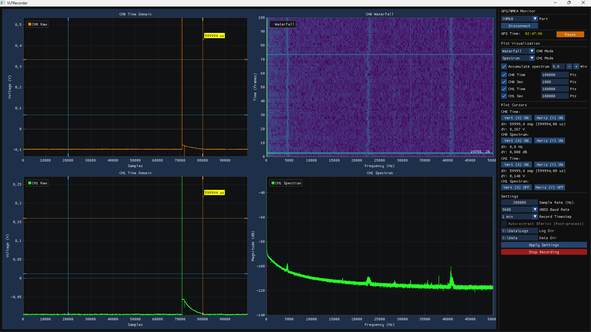
Interface

The interface is organized around the operator’s workflow.
The left side contains the CH0/CH1 time-domain views.
The central area provides waterfall and spectrum visualization.
The right-hand control area contains:
- GPS/NMEA status;
- acquisition settings;
- sample-rate configuration;
- GNSS serial configuration;
- recording timestep;
- data and log directories;
- visualization controls;
- cursor readouts.
The result is a single workstation view combining acquisition status, signal inspection, timing state, and recording configuration.
Timing architecture across projects
VLFRecorder is part of a broader timing-related engineering approach.
The same GPS-PPS discipline appears in the separate PPS timing system project.
There, PPS timing was characterized between two GNSS receivers using an STM32 timer.
Here, the same general timing concept is applied at a different level:
- PPS provides the external timing event;
- GPSDO provides the acquisition clock;
- the DAQ hardware uses those references directly;
- GPS time determines session boundaries and timestamps.
The two projects therefore address different layers of the same problem.
The PPS timing project examines the behavior of the timing reference itself.
VLFRecorder uses that reference as part of a complete acquisition and recording system.
What the project demonstrates
Although VLFRecorder is a specific station application, the engineering problems it addresses are broader than VLF monitoring.
The project combines several areas that normally appear as separate subsystems:
Hardware interfacing
Direct communication with a dedicated USB DAQ and configuration of external clock and trigger inputs.
Real-time acquisition
Continuous asynchronous acquisition with a finite processing deadline and double buffering.
Multithreaded software
Independent acquisition, visualization, GPS parsing, and statistics/session-management workers, coordinated through scoped locks and atomics rather than a single shared mutex.
Digital signal processing
FFT-based spectral analysis, waterfall generation, envelope construction, statistical thresholding, and event extraction.
Time synchronization
Using GPSDO/PPS at the hardware level and GPS-derived time at the recording/session level.
Data engineering
Binary session files, explicit headers, sample counts, automatic rotation, and post-processing.
Reliability engineering
Explicit handling of missing synchronization, stale GPS state, acquisition errors, and unattended operation.
Operator tooling
Live visualization, measurement cursors, configurable rendering, and non-destructive display pause.
The interesting part is not any single feature.
It is the interaction between them.
A typical operating cycle
A normal unattended session can be summarized as:
1. Start application
↓
2. Establish GPS/GNSS communication
↓
3. Wait for valid GPS state
↓
4. Synchronize DAQ acquisition to external PPS
↓
5. Start continuous 200 kHz acquisition
↓
6. Process incoming buffers
↓
7. Update live CH0/CH1 visualization
↓
8. Record binary session data
↓
9. Monitor GPS state and sample counts
↓
10. Rotate the session at the GPS minute boundary or sample-count limit
↓
11. Optionally run sferic extraction on the completed session
↓
12. Continue with the next session
The operator can inspect the live data without interrupting this pipeline.
What’s next
The planned additions at the time of writing are focused on reducing the remaining points of manual intervention.
Manual event markers
Allow the operator to place event markers directly on the live plots during monitoring.
This would preserve human observations alongside automatically detected events.
Acquisition watchdog
Add a watchdog capable of detecting and recovering from a DAQ connection or GPS-link failure during unattended operation.
The goal is to move another class of recoverable faults from:
operator notices → operator diagnoses → operator restarts
toward:
system detects → system recovers → system logs the event.
Design principles
Several principles ended up shaping the system repeatedly.
Hardware timing should stay hardware timing
If the timing reference is available at the hardware level, there is little reason to recreate it through host software.
Acquisition should be boring
The most important part of the system is the part that should attract the least attention during normal operation.
Samples should arrive, be processed, and be recorded without the UI becoming part of the critical path.
Visualization is a consumer, not the source of truth
The live display exists to help an operator understand the data.
It should never determine whether the underlying acquisition continues.
Fail explicitly
A missing GPS reference should not look like valid data.
A failed connection should be logged.
A stale timestamp should not silently become a trustworthy timestamp.
Separate raw data from interpretation
Continuous recording preserves the underlying signal.
Sferic extraction and visualization operate on top of that data.
This allows analysis methods to evolve without changing the fundamental acquisition layer.
Isolate what fails independently
Serial state, sample buffers, and the session-file writer are kept behind separate locks, and the flags that cross thread boundaries most often are atomics rather than mutex-guarded fields. A slow disk, a jittery serial link, or a busy UI frame should each be contained to its own subsystem rather than able to stall the acquisition thread.
A note on the source
The source code of VLFRecorder is the property of the Institute of Solar-Terrestrial Physics, Siberian Branch of the Russian Academy of Sciences (ISTP SB RAS), and is not publicly available.
The purpose of this write-up is therefore not to reproduce the implementation, but to document the system architecture, acquisition strategy, synchronization design, processing pipeline, and engineering decisions behind the application.