Overview
A follow-up to the VLF recorder work — a parallel project at the Institute characterizing PPS (pulse-per-second) timing accuracy across two GNSS receivers, both running in survey-in mode: a u-blox NEO-M8T and a ZED-F9T.
The question was straightforward:
How precisely can the PPS outputs of two GNSS receivers be compared, and how much of the measured jitter actually comes from the measurement system itself?
The idea is simple on paper: capture each receiver’s PPS edge on a hardware timer, compare timestamps, and calculate the timing variation.
In practice, getting there meant fighting the measurement system itself for a while — a clock tree misconfiguration, and a HardFault buried behind a stale debugger session.
None of that shows up as “wrong data”.
It shows up as the board simply not booting.
Once the embedded system was working reliably, the experiment became a much simpler problem: build a measurement chain whose own timing uncertainty was small enough that the receivers’ jitter could actually be observed.
Hardware setup
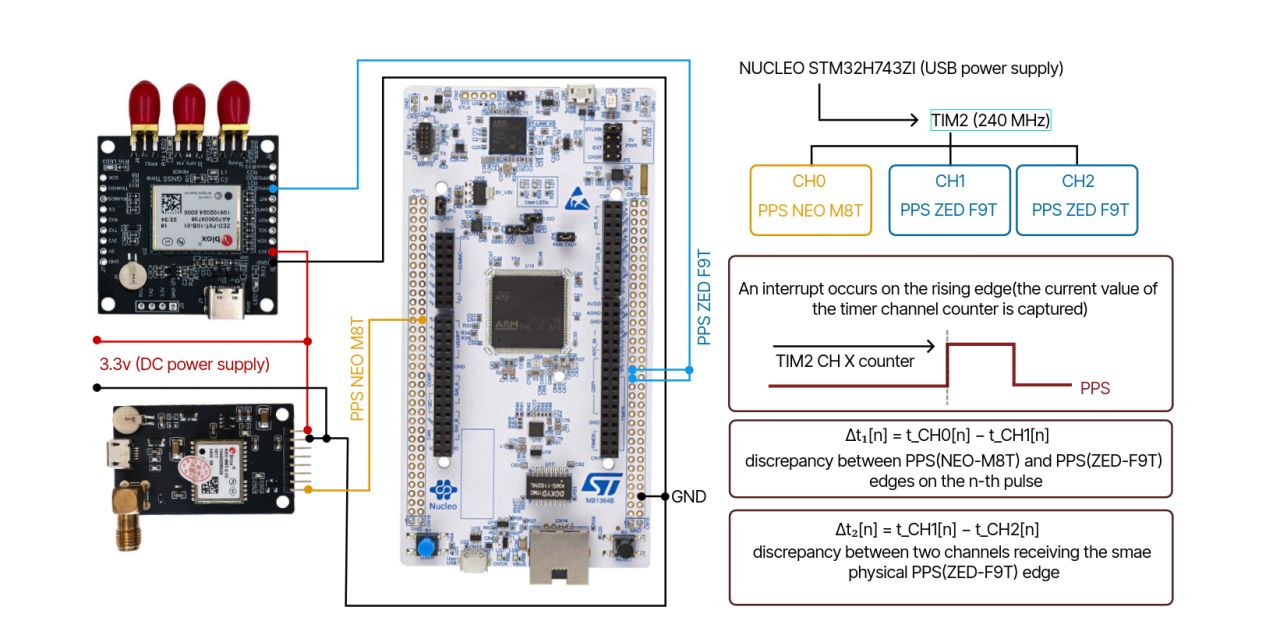
The final measurement system was built around an STM32H743 Nucleo-144 board.
- MCU: STM32H743
- Timer: TIM2
- Timer clock: 240 MHz
- Input capture: 3 channels
- Receiver 1: u-blox NEO-M8T PPS
- Receiver 2: u-blox ZED-F9T PPS
The three input-capture channels were used as follows:
- one channel captured the NEO-M8T PPS edge;
- one channel captured the ZED-F9T PPS edge;
- the third channel was connected to the same ZED-F9T PPS edge as the second channel.
That last part is intentional.
It provides a way to measure the timing variation introduced by the measurement system itself.
NEO-M8T PPS ───────────────> TIM2 input capture CH1
                                  │
ZED-F9T PPS ────────┬──────────> TIM2 input capture CH2
                    │
                    └──────────> TIM2 input capture CH3
                     STM32H743
                     TIM2 @ 240 MHz
The two channels connected to the same physical PPS edge should, ideally, see exactly the same event.
Any measured difference between them therefore cannot be receiver-to-receiver timing error.
It is a measurement of the system’s own timing floor.
Why measure the system floor?
If the two receivers are compared directly, the measured variation contains more than just receiver jitter.
Conceptually:
\[ \sigma_\mathrm{measured}^2 = \sigma_\mathrm{receiver}^2 + \sigma_\mathrm{system}^2 \]The measurement system therefore needs to be characterized separately.
That is why two timer channels were connected to the same ZED-F9T PPS output.
This gives a direct estimate of the timing uncertainty introduced by the capture system itself.
Without that control measurement, a few nanoseconds of measured variation could not be confidently attributed to the receivers.
Measurement method
The experiment ran for approximately 24 hours, recording one PPS event per second.
That gives a long sequence of hardware-captured timestamps rather than relying on software timestamps.
The important part is where the timestamp is generated.
The PPS edge is captured directly by the timer hardware. The timestamp is therefore latched by the peripheral at the event itself rather than being generated later by code running in the main loop.
In other words:
This matters because software execution time and main-loop load should not become part of the timing measurement.
The experiment is therefore measuring the timing of the input edges, not the response time of the firmware.
Debugging the measurement system
Before collecting useful data, the measurement system itself had to become trustworthy.
The first problems were not subtle timing errors.
The board simply would not behave as expected.
A clock-tree configuration problem prevented the timer from operating with the intended clock, while a HardFault was initially obscured by a stale debugger session.
These failures were useful reminders of an important property of measurement systems:
A broken measurement chain does not necessarily produce obviously broken data.
It can also produce nothing at all — or, worse, data that looks reasonable but cannot be trusted.
For this experiment, the timer configuration and capture path therefore had to be established before interpreting the statistical results.
Firmware implementation
The measurement chain described above is not just “start input capture and read a callback.” A few implementation details turned out to matter enough that they’re worth documenting alongside the results — the full source is linked at the end of this post.
Capturing in the ISR, not the HAL callback
TIM2_CaptureIRQHandler() reads TIM2->CCR1 / TIM2->CCR3 directly out of
the timer’s status register, instead of going through
HAL_TIM_IC_CaptureCallback(). The timer already latches the capture value
in hardware the instant the edge arrives — that part is exact regardless of
software. What isn’t automatically exact is turning a 32-bit hardware
counter into a 64-bit timestamp that survives a multi-hour run without
wrapping.
uint32_t ovf = tim2_ovf;
if (update_pending) {
    tim2_ovf = ovf + 1u;
}

/* Guard against the capture/overflow race on the wrap boundary
 * (~once every 17.9 s at 240 MHz / 32-bit ARR): if update just fired
 * and CCRx is small, the capture happened AFTER the wrap, so the
 * high word must be ovf+1 rather than the pre-update ovf. */
if (got1) {
    uint32_t use_ovf = (update_pending && cap1 < OVF_GUARD) ? ovf + 1u : ovf;
    fifo_push(&fifo1, ((uint64_t)use_ovf << 32) | cap1);
}
The 32-bit counter at 240 MHz wraps roughly every 17.9 seconds. Every wrap
sets the update flag and increments a software overflow counter. The one
case that needs explicit handling is a capture landing right at the wrap
boundary — did the edge happen just before the rollover (still belongs to
the old overflow count) or just after (belongs to the new one)? OVF_GUARD
resolves that ambiguity by checking whether the captured value is
suspiciously small at the same instant the update flag is set.
Two FIFOs, and why they need to talk to each other
Each channel gets its own ring buffer (fifo1, fifo3). That part is
unremarkable. What isn’t obvious until it happens: if one channel’s queue
falls behind the other by even a single edge — for instance because the
UART transmit in the main loop briefly blocked while a serial terminal
wasn’t reading fast enough — naively popping “the front of each queue” now
pairs a timestamp from PPS edge N on one channel with edge N+1 on the
other. The reported delta doesn’t look obviously wrong; it just jumps to
roughly one whole PPS period (plus the real jitter, which is now buried
under it), and it never self-corrects.
static int align_fifos(void)
{
    for (;;) {
        uint64_t t1, t3;
        if (!fifo_peek(&fifo1, &t1)) return 0;
        if (!fifo_peek(&fifo3, &t3)) return 0;

        uint64_t newest = (t3 > t1) ? t3 : t1;

        int aligned = 1;
        if (newest - t1 > PPS_RESYNC_THRESHOLD_TICKS) { fifo_drop_front(&fifo1); aligned = 0; }
        if (newest - t3 > PPS_RESYNC_THRESHOLD_TICKS) { fifo_drop_front(&fifo3); aligned = 0; }

        if (aligned) return 1;
    }
}
align_fifos() peeks both queues without consuming them, and discards
whichever side is stale by more than half a PPS period before the main loop
is allowed to pop a pair. This is the part of the firmware that keeps a
24-hour CSV trustworthy from the first sample to the last, rather than only
for the first few seconds before anything in the system has a chance to
hiccup.
The HardFault, in retrospect
Earlier in this post: “a HardFault was initially obscured by a stale debugger session.” Here’s what was actually going on underneath that.
The original version of this firmware formatted timestamps with
snprintf() and a %llu specifier for the 64-bit values. That’s a
reasonable thing to reach for — and it’s also a landmine on this specific
toolchain. STM32CubeIDE links against newlib-nano by default, which is
commonly built without long long support in the printf family. A
%llu specifier in that configuration doesn’t just print the wrong number.
It desyncs the internal va_list walk, so every argument after the
mismatched one gets read from the wrong stack offset — and when a later
%s in the same format string dereferences whatever garbage pointer
happened to land there, that’s a HardFault that has nothing to do with the
timer, the GPIO, or the clock tree. It looks exactly like “the board is
broken,” which is precisely why it was confusing to chase down at first.
The fix was to stop using the printf family entirely for this:
static void format_ns(int64_t ticks, char *out, size_t outsz)
{
    char *p = out;
    if (ticks < 0) { *p++ = '-'; ticks = -ticks; }
    uint64_t num = (uint64_t)ticks * 25000ULL;
    uint64_t value_x1000 = (num + 3ULL) / 6ULL;   /* round half up */
    uint64_t ns_int  = value_x1000 / 1000ULL;
    uint64_t ns_frac = value_x1000 % 1000ULL;

    p += u64_to_dec(ns_int, p);
    *p++ = '.';
    if (ns_frac < 10)       { *p++ = '0'; *p++ = '0'; p += u64_to_dec(ns_frac, p); }
    else if (ns_frac < 100) { *p++ = '0'; p += u64_to_dec(ns_frac, p); }
    else                     { p += u64_to_dec(ns_frac, p); }
    *p = '\0';
}
Hand-rolling the tick-to-nanosecond conversion (240 MHz → 25/6 ns per tick, done here as integer fixed-point math to avoid pulling in float formatting too) removes the entire class of bug. There’s no format string to misinterpret, and the timing of the conversion itself is fully deterministic — which matters slightly less for correctness here and a lot more for not second-guessing whether formatting overhead is contaminating anything downstream.
Input capture filter
sConfigIC.ICFilter = 0x3;
This requires roughly six consecutive samples at the timer’s sampling clock (~25 ns at 240 MHz) before an edge is accepted, which rejects short glitches without affecting real PPS edges — those rise cleanly and hold far longer than 25 ns. It’s applied identically to both channels, so the fixed filter delay is common-mode and cancels out in the CH1-vs-CH3 delta instead of biasing it.
Timer resolution
With TIM2 running at 240 MHz, one timer tick corresponds to:
\[ T_\mathrm{tick} = \frac{1}{240\,\mathrm{MHz}} \approx 4.167\,\mathrm{ns} \]So the timestamp quantization step is approximately 4.167 ns.
This limitation is visible directly in the recorded data.
The measured timing differences do not form a perfectly continuous distribution. Instead, the values show discrete steps associated with the timer’s finite resolution.
This is an important distinction:
Timer resolution is not the same thing as measurement jitter.
The timer defines the granularity with which an edge can be represented. The statistical spread of the captured timestamps is the quantity being characterized.
Results
The 24-hour run produced three useful measurements:
| Measurement | σ |
|---|---|
| Channel-to-channel, same PPS edge (system floor) | ≈ 1.6 ns |
| NEO-M8T vs ZED-F9T (raw) | ≈ 7.5 ns |
| Receiver-to-receiver jitter, system floor removed | ≈ 7.3 ns |
The first number is the measurement system’s own timing floor.
The second is what is observed when the two different receivers are compared.
The third attempts to isolate the receiver contribution by removing the independently measured system contribution.
Removing the measurement-system floor
The system-floor measurement was approximately:
\[ \sigma_\mathrm{system} \approx 1.6\,\mathrm{ns} \]while the direct NEO-M8T vs ZED-F9T comparison gave:
\[ \sigma_\mathrm{measured} \approx 7.5\,\mathrm{ns} \]Assuming the two contributions are independent, their variances add:
\[ \sigma_\mathrm{measured}^2 = \sigma_\mathrm{receiver}^2 + \sigma_\mathrm{system}^2 \]Therefore:
\[ \sigma_\mathrm{receiver} = \sqrt{ \sigma_\mathrm{measured}^2 - \sigma_\mathrm{system}^2 } \]Substituting the measured values:
\[ \sigma_\mathrm{receiver} = \sqrt{ 7.5^2 - 1.6^2 } \]\[ \sigma_\mathrm{receiver} \approx 7.33\,\mathrm{ns} \]or approximately:
The correction is relatively small because the measurement system floor is much smaller than the observed receiver-to-receiver variation.
What the data actually shows
The result is not just a single standard-deviation number.
The distribution also contains visible quantization steps corresponding to the approximately 4.167 ns timer resolution.
That gives an additional sanity check on the measurement chain.
The hardware is behaving like a finite-resolution timestamping system should behave.
The measured distribution therefore contains two different things:
- Physical timing variation from the signals being compared.
- Quantization introduced by the timer used to timestamp those signals.
Keeping those two effects conceptually separate is important when interpreting nanosecond-scale measurements.
Capture plots
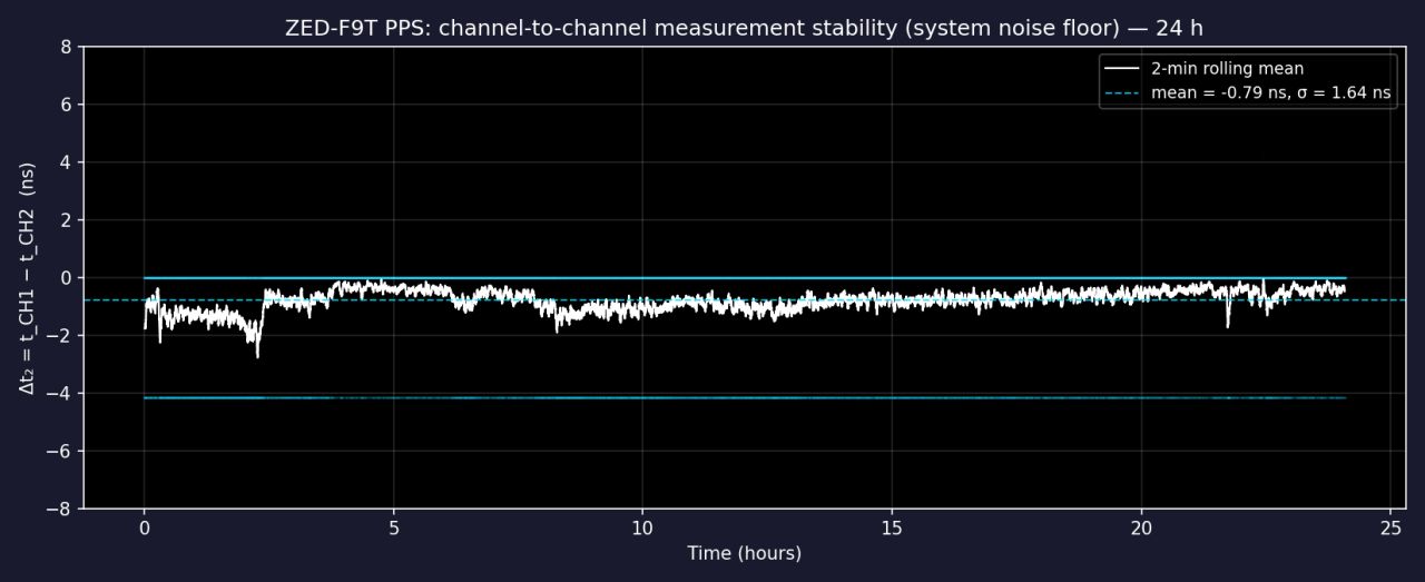
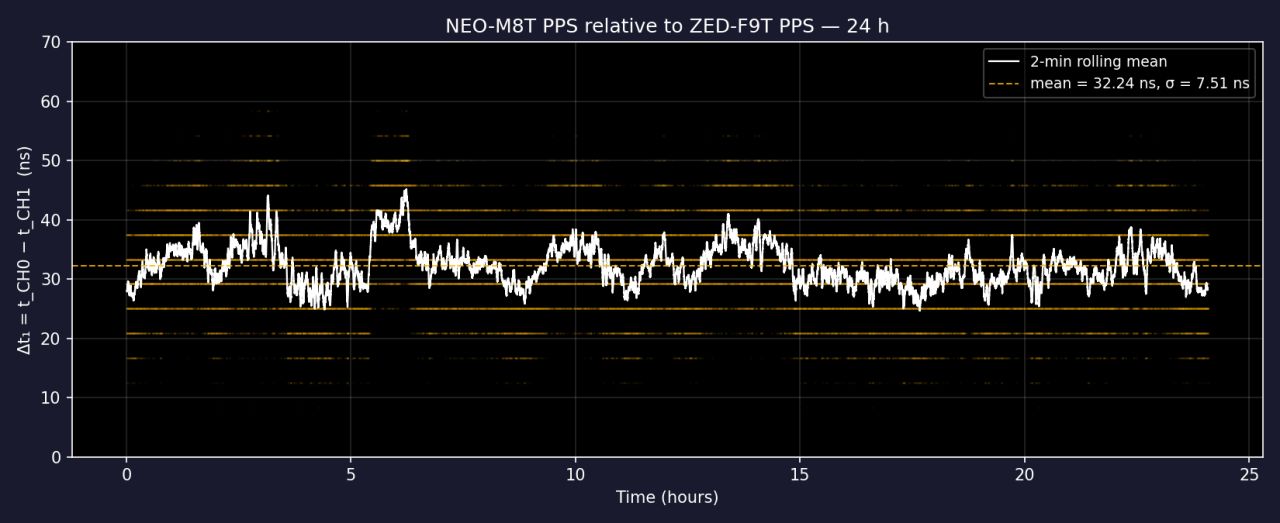
The two plots answer different questions.
The receiver comparison shows the variation observed between the two independent PPS sources.
The same-edge comparison shows how much variation is introduced even when the physical PPS event is identical.
That second measurement is what makes the first result interpretable.
Validation
The most useful outcome of the experiment was not simply obtaining a number around 7 ns.
It was obtaining a number that is consistent with the expected performance of the receivers.
The measurement chain produced:
- approximately 1.6 ns of system-level variation when measuring the same PPS edge;
- approximately 7.5 ns when comparing the two receivers;
- approximately 7.3 ns after removing the independently measured system floor.
The resulting receiver-to-receiver figure is in line with the relevant receiver specifications.
That agreement is the important validation.
A timing experiment can always produce a plausible-looking distribution.
The harder question is whether the measurement chain is actually capable of producing a trustworthy result.
Here, the independently measured system floor, the observable timer quantization, and the resulting receiver comparison all provide evidence that the measurement chain is behaving consistently with its expected limitations.
What I would change in a second version
The experiment also exposed a few limitations of the current setup.
The timer resolution is approximately 4.167 ns, so the timestamp representation is already coarse compared with the final jitter number.
A future version could therefore improve the timestamping resolution and investigate the remaining quantization contribution more directly.
The current experiment was also designed primarily to establish a trustworthy comparison between the two receivers.
A more extensive characterization would separate additional sources of variation and examine how the result changes with different receiver configurations and operating conditions.
For the original question, however, the measurement chain was sufficient:
the two receivers could be compared, the system floor could be measured independently, and the resulting timing variation landed in the expected nanosecond range.
Takeaway
The interesting part of this experiment was not getting a nanosecond number out of an STM32.
It was building a measurement system where that number could actually be trusted.
The chain ended up being:
Final result: ≈ 7.3 ns receiver-to-receiver jitter.
More importantly: the measurement system had a separately characterized floor of approximately 1.6 ns, and the timer’s 4.167 ns quantization was visible in the recorded data.
That is what makes the result useful rather than merely plausible.
Code
The full STM32CubeIDE project — ISR capture, the FIFO alignment logic, and the printf-free timestamp formatting — is on GitLab: