Overview
IONOSPHERE_PRO is a web dashboard and processing pipeline for a small network of ground stations that measure ionospheric total electron content (TEC) by tracking the coherent dual-frequency beacon transmitted by the Ionosfera-M satellite pair. Each station records raw IQ samples at 150 MHz and 400 MHz during a satellite pass; the backend turns those recordings into phase and TEC curves; the frontend presents all of it as a live map with a per-station history of processed sessions.
It’s the software layer that sits between “two SDR receivers pointed at the sky” and “a scientist looking at a TEC curve” — ingest, signal processing, storage, auth, and visualization, built as one coherent system rather than a pile of one-off scripts.
The source code is the property of the Institute of Solar-Terrestrial Physics, Siberian Branch of the Russian Academy of Sciences (ISTP SB RAS), and is not publicly available. This write-up describes the architecture, the measurement technique, and the engineering decisions behind the application without reproducing any part of the implementation.
The measurement technique
Ionosfera-M transmits two phase-coherent tones, at 150.048 MHz and 400.128 MHz — the same technique used by classic ionospheric beacon satellites for decades. Because both tones originate from the same onboard oscillator, their frequencies are locked in an exact 3:8 ratio. As the signal passes through the ionosphere, the two frequencies pick up different amounts of phase delay from the same electron content along the path — the delay is frequency-dependent. Scale the 400 MHz phase down by 3/8 and subtract it from the 150 MHz phase, and what’s left is a curve proportional to the total electron content the signal traversed. Everything else about the pipeline exists to get from raw IQ samples to that one subtraction cleanly.
There’s a second signal buried in the same recording: the satellite’s own along-track velocity imposes a large, smoothly varying Doppler shift on both tones — tens of kilohertz over the few minutes of a pass, following the characteristic S-curve shape of a near-overhead LEO pass (v0 - A·tanh(k·(t − t_close)), a good fit for the along-track geometry near closest approach). That Doppler shift has to be estimated and removed before the TEC subtraction means anything, because it dwarfs the phase perturbation caused by the ionosphere itself.
Signal processing pipeline
Each recorded pass goes through the same sequence, per station, per satellite:
raw IQ (150 MHz + 400 MHz) → coarse Doppler fit → residual Doppler tracking → coherent demodulation & integration → phase unwrap → 150/400 differencing → relative TEC
Coarse Doppler: fitting the pass geometry
The 400 MHz channel is chopped into short windows, and the FFT peak frequency in each window is tracked over the whole pass. That noisy peak-frequency trace gets a median filter, then a least-squares fit to the tanh model above (scipy.optimize.leastsq). The result is a smooth prediction of the pass’s bulk Doppler at any point in time, driven by orbital geometry rather than by tracking noise sample-to-sample.
Residual Doppler: what the coarse fit misses
The tanh fit captures the geometric trend but not everything — receiver oscillator drift, finer structure the model doesn’t cover. So a second pass repeats the FFT-peak-tracking idea on 200 evenly spaced windows across the recording, this time after subtracting the coarse model, and interpolates the leftover (residual) frequency into a continuous function of time.
Coherent demodulation
With both a coarse and a residual Doppler estimate, every short window of both channels gets mixed down by the combined predicted Doppler for that instant, then coherently accumulated. This is the computationally heavy part of the pipeline — a complex mix-and-sum over every sample in the recording — and it’s implemented twice:
- a GPU path (CuPy), vectorized across the whole batch of windows at once, used when a CUDA device is available (developed against an RTX 3060);
- a CPU path (Numba,
@njit(parallel=True)), used automatically whenever the GPU path is unavailable or throws at runtime — the code tries GPU first and falls back to CPU inside the same batch loop, so a machine without a GPU, or a GPU that fails for any reason mid-run, degrades to CPU rather than crashing the session.
From phase to TEC
The accumulated complex values for each window are unwrapped in phase (np.unwrap(np.angle(...))) to give continuous phase-vs-time curves for both channels. The 400 MHz phase is scaled by 3/8 and subtracted from the 150 MHz phase — that difference is the relative TEC curve. All three curves (150 MHz phase, 400 MHz phase, relative TEC) are rendered and saved as the output of a processed session.
From desktop script to a multi-station service
The processing code didn’t start life as a service. The original version (graph.py) had station, satellite, and file names hardcoded in a Main() function, and it printed a RESULT_JSON: line to stdout specifically so a wrapping Electron desktop app could parse it — a single-operator, single-machine tool.
Turning that into something a network of stations could share meant lifting every hardcoded assumption into a parameter: which station, which pass, which pair of IQ files, and — importantly — where the output goes. The reworked entry point (process_session.py) takes station ID and file paths as arguments and writes its output into a predictable, self-describing layout:
data/<station_id>/sessions/<session_id>/meta.json
data/<station_id>/sessions/<session_id>/tec.png
data/<station_id>/sessions/<session_id>/phase150.png
data/<station_id>/sessions/<session_id>/phase400.png
That structure is the entire contract between the processing script and the web backend — the backend never needs to know anything about Doppler models or coherent integration, only how to walk a directory of meta.json files. New stations, in principle, need nothing more than a new entry in a station registry and a place on disk for their sessions to land; the processing and serving code doesn’t change.
Backend and API
The Flask backend is deliberately thin on top of that file layout. A station registry (stations.json — id, name, coordinates, description, the satellite names it targets) is the source of truth for what’s on the map; a small manage_users.py CLI hashes passwords into users.json for the handful of named operator accounts, checked against on login and exchanged for a JWT.
From there, the API is close to a direct read of the session directory structure:
GET /api/stations— the registry, each entry annotated with its most recent session’s metadata so the frontend can show which stations have recent data;GET /api/stations/<id>/sessions— that station’s session history, newest first;GET /api/stations/<id>/sessions/<session_id>— one session’s metadata;GET /api/data/<id>/<session_id>/<filename>— the actual plot images.
The one deliberate wrinkle: <img> tags can’t send an Authorization header, so the JWT library is configured to also accept the token as a ?token= query parameter, and the frontend appends it when building plot URLs. Everything else stays on bearer-token auth in the header.
Satellites are a separate, honest layer
Ground stations are fixed points; satellites are not, and the frontend treats them accordingly — two different overlays on the same map rather than one blurred concept. GET /api/satellites reads the target satellite names out of the station registry, resolves them against current TLE data (Skyfield/SGP4), and returns a short predicted ground track for each. A companion GET /api/satellites/debug endpoint reports exactly how many TLEs loaded, which targets matched, which didn’t, and where the TLE data actually came from — useful precisely because “the map shows no satellites” is otherwise a silent failure with several unrelated possible causes (bad TLE fetch, a name that doesn’t match what’s in the station registry, an empty TLE set), and staring at an empty overlay doesn’t tell you which one it was.
Frontend
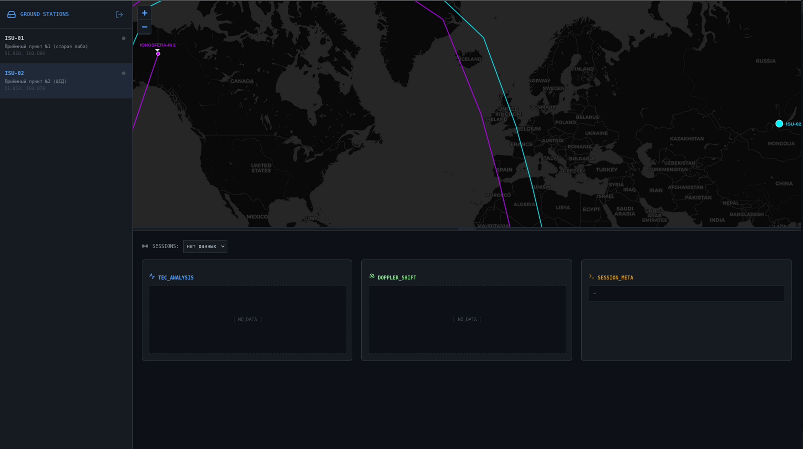
The interface is a single-page dark-themed dashboard: a station list on the left, a resizable map/session-panel split filling the rest.
- The map (Leaflet) shows every registered station as a marker, colored by whether it has produced a session in the last 24 hours, plus the live satellite ground tracks as a separate overlay with its own color per satellite.
- Selecting a station loads its session history into a panel below the map, each session showing the processed phase/TEC plots for that pass.
- The map/panel split is user-resizable by dragging a divider, rather than a fixed layout — a small feature, but one that matters when a plot needs more room than the default split gives it.
The API client uses a relative base URL (API_BASE = ''), so the frontend, once built, is just static assets that work regardless of what host or port they’re served from — a small design choice that turned out to remove an entire category of deployment complexity later (more on that below).
Deployment: running unattended on an air-gapped machine
The central server this runs on has no outbound internet access at all, is reachable only through a chain of SSH jump hosts and a NAT port forward, and is operated by someone who isn’t a developer — so the whole stack had to reduce to “copy one archive over, run one script.”
That constraint ruled out the obvious approach (pip install from a wheelhouse on the target) outright: the target doesn’t even have python3-venv installed, and can’t install it without the apt access it doesn’t have. The solution was to do all dependency resolution on a machine with internet — resolve the full dependency graph, download each package individually pinned to the target’s exact platform/ABI (one at a time, since a batch pip download under a platform restriction silently fetches nothing if even one package lacks a matching wheel), and unpack the resulting wheels directly into a vendor/ folder. On the target, there’s no install step at all: PYTHONPATH=./vendor python3 app.py, nothing to compile, nothing to activate. The one dependency with no prebuilt wheel — a small pure-Python package — gets built locally as a py3-none-any wheel, which runs anywhere regardless of what machine built it.
That, plus the fact that the frontend already used a relative API base URL, removed the need for nginx as well — Flask serves the built React assets directly via a catch-all route registered after the API routes, so one process on one port handles everything. TLS on that port is a self-signed certificate (no ACME/CA reachable from an air-gapped host), fine for a handful of named operators who click through one browser warning.
The harder lessons were less about the happy path and more about failure modes that only show up once a service is meant to run unattended:
- A first version supervised the process with
nohup ... &, which survives a closed SSH session but not much else — nothing restarts a process that crashes, and nothing brings it back after a reboot. Worse, the liveness check (kill -0 $PID) turned out to lie in two different ways: a dead process’s PID gets recycled by the OS, sokill -0on a stale PID can report “alive” for a completely unrelated process; and a PID file owned byrootmakeskill -0fail with a permission error that’s indistinguishable, from a plain shell check, from “no such process.” Both problems disappeared by handing supervision tosystemd(Restart=always, enabled at boot) and askingsystemctlfor status instead of reasoning about/procby hand. - The app fetches fresh satellite TLE data from CelesTrak at startup. On a network that actively refuses the connection, that fails fast; on a genuinely air-gapped network — no route, just silence — an unbounded socket call can hang for the OS-level TCP timeout, stalling every single startup. A five-second
socket.setdefaulttimeout()scoped around just that call, paired with a local TLE snapshot fallback, bounds the worst case regardless of which kind of “no network” it turns out to be. - The most expensive bug wasn’t a crash at all — it was a redeploy that came back up in Flask’s debug mode, on plain HTTP, because the bundle had been rebuilt from an older, unmodified copy of the source tree rather than the current one. A “working” service running the wrong build is a more dangerous failure mode than an obviously broken one, since nothing about its outward behavior flags it — that’s what pushed the deploy script toward an explicit startup self-check (do the vendored imports actually resolve?) rather than trusting that “the process came up” means “the correct process came up.”
What the project demonstrates
IONOSPHERE_PRO touches several areas that normally live in separate subsystems, tied together end to end:
Radio physics and signal processing — coherent dual-frequency demodulation, Doppler curve fitting against real pass geometry, and a differential-phase TEC derivation, implemented with a GPU path and an automatic CPU fallback for the heavy numerical core.
System design that mirrors the data’s own shape — a session directory layout (data/<station>/sessions/<id>/) that is the contract between the offline processing script and the web backend, letting new stations plug in without touching either side’s code.
A small, honest API surface — read-mostly endpoints that map closely onto that directory structure, plus a debug endpoint built specifically to make an otherwise-silent failure (an empty satellite overlay) diagnosable instead of mysterious.
A frontend that treats different kinds of geography differently — fixed ground stations and moving satellite tracks as two distinct map layers, rather than one blurred concept, because they behave differently and an operator needs to reason about them differently.
Deployment engineering for a machine that starts from zero — no outbound internet, no guaranteed pip/venv, no CA, run by a non-developer. Getting a real scientific tool to run reliably and unattended there meant re-deriving several things (dependency installation, process supervision, TLS trust, network failure handling) that a normal deployment gets for free.
Design principles
The output format is the interface
process_session.py and the Flask backend never share code, a queue, or an RPC boundary — just a directory structure. That’s a small, boring, very robust integration point precisely because it’s just files.
GPU is an optimization, not a requirement
The coherent-integration core has two implementations behind one call site, and the code decides which one to use at runtime rather than at deploy time. A missing or misbehaving GPU degrades performance, not correctness.
Nothing installs on the target
If a dependency can be fully resolved and unpacked ahead of time, there is no reason to give a machine you can’t easily walk up to an installer to run at all.
Fail loudly, not gracefully, when something foundational is missing
An empty satellite overlay, a silently-empty TEC plot, or a service that “looks running” but isn’t the build you tested are all worse than an explicit error, because none of them tell the operator anything is wrong.
The deployed artifact and the reviewed artifact must be provably the same thing
A working-but-wrong deployment (right process, wrong source tree) is more dangerous than a broken one, because nothing about its outward behavior flags it.
A note on scope
This is an internal tool built for a small network of monitoring stations at a research institute, not a public product — there’s no public repository, and this write-up describes the architecture, the measurement technique, and the engineering decisions rather than reproducing implementation details.