Putting the Hantek DSO2D10 on a Python leash

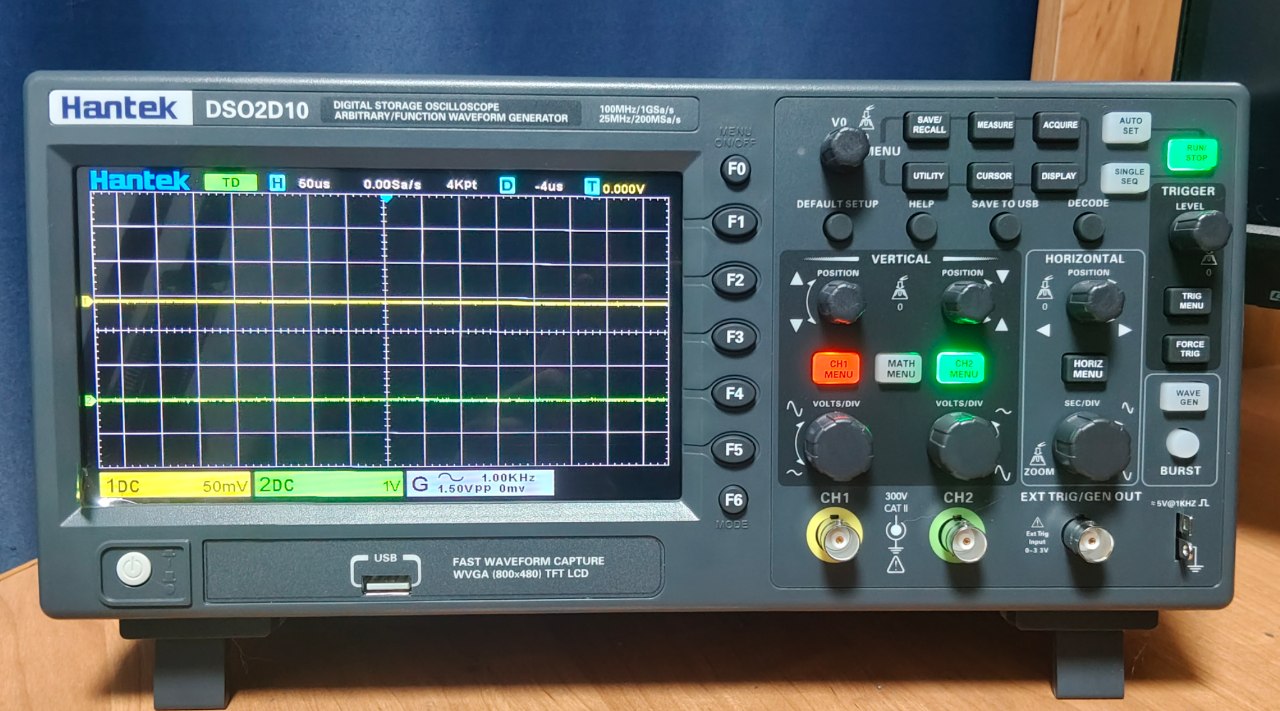
A friend from Belarus Alex gave me a Hantek DSO2D10.

Naturally, the first thing I did was try to make it talk to Python.

What makes this interesting is not just remote control of the instrument, but the possibility of making the oscilloscope part of a programmable measurement system. The scope can be controlled from Python, its built-in signal generator can be operated programmatically, and captured waveform data can be transferred back to the computer for further processing.

That makes experiments such as automated frequency-response measurements possible. Instead of manually changing the generator frequency, reading the amplitude and phase from the screen, and writing the results down, a script can perform the whole measurement and produce the resulting data automatically.

This is also where a digital oscilloscope becomes particularly interesting for laboratory work. A student can spend less time repeating routine measurements and more time working with the actual signal-processing problem. Once the samples are in Python, they are no longer tied to the oscilloscope’s built-in measurements either: FFT, filtering, averaging, spectral analysis, or completely custom processing can be implemented independently. Captured waveforms can also be saved and replayed later as test data.

So I wanted to see how far I could get without a vendor-specific software stack and whether the DSO2D10 could be turned into a reasonably open measurement instrument.

The setup is fairly simple: Debian 13, the scope connected over USB, and Python talking directly to the Linux USBTMC device at /dev/usbtmc1.

There is one slightly annoying detail: at the moment I have to give the device permission manually:

sudo chmod +x /dev/usbtmc1

Then the scope can be opened directly from Python without a VISA stack:

fd = os.open("/dev/usbtmc1", os.O_RDWR)

os.write(fd, b"*IDN?\n")
response = os.read(fd, 4096)

print(response)

The first test worked:

b'undefined, DSO2D10, undefined, 3.0.0(240326.00)'

From there I started querying the instrument and experimenting with its waveform interface:

:ACQuire:POINts?
:WAV:FORM?
:WAV:SOUR?
:WAVeform:DATA:ALL?

The interesting part was figuring out what actually comes back from :WAVeform:DATA:ALL?.

The DSO2D10 does not simply return one convenient block of samples. The waveform arrives as packets with a 29-byte header containing the packet size, total data size and position of the packet in the complete buffer.

For a 4000-point acquisition, the scope returned two packets:

packet 1:
    packet size = 128
    position    = 0
    payload     = 99 bytes

packet 2:
    packet size = 4029
    position    = 99
    payload     = 4000 bytes

The first 99 bytes appear to be metadata. The remaining 4000 bytes contain the waveform data.

I reconstruct the complete buffer using the position field from each packet:

buffer = bytearray(total_size)

for packet in packets:
    position = packet["position"]
    payload = packet["payload"]

    buffer[
        position:position + len(payload)
    ] = payload

The complete test script is available in the tools repository.

There was also a small surprise here.

The waveform was requested using:

:WAV:FORM WORD

so my first assumption was that 4000 points should produce 8000 bytes of waveform data.

It doesn’t.

The instrument returned exactly 4000 bytes:

4000 points
4000 waveform bytes

The raw payload starts with values such as:

02 02 03 03 02 02 02 03 02 03 ...

For now I’m treating these as one-byte samples and inspecting the resulting waveform in NumPy rather than assuming that WORD necessarily means a conventional 16-bit sample representation.

The raw waveform can then be pulled directly into NumPy:

samples = np.frombuffer(
    waveform_bytes,
    dtype=np.uint8
)

and plotted with Matplotlib.

The reconstructed waveform can be compared directly with the signal shown on the oscilloscope:

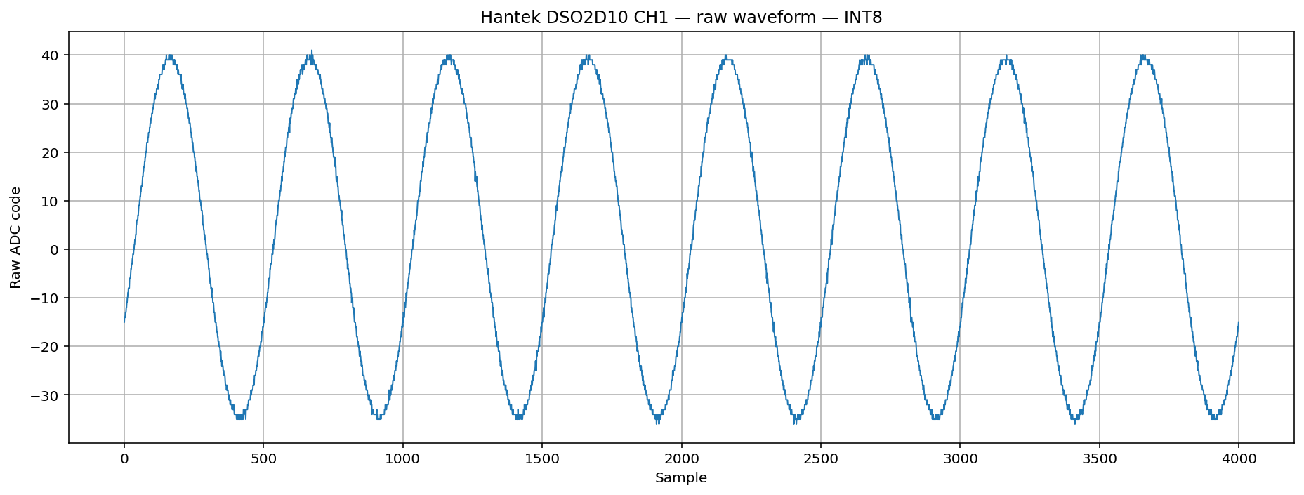
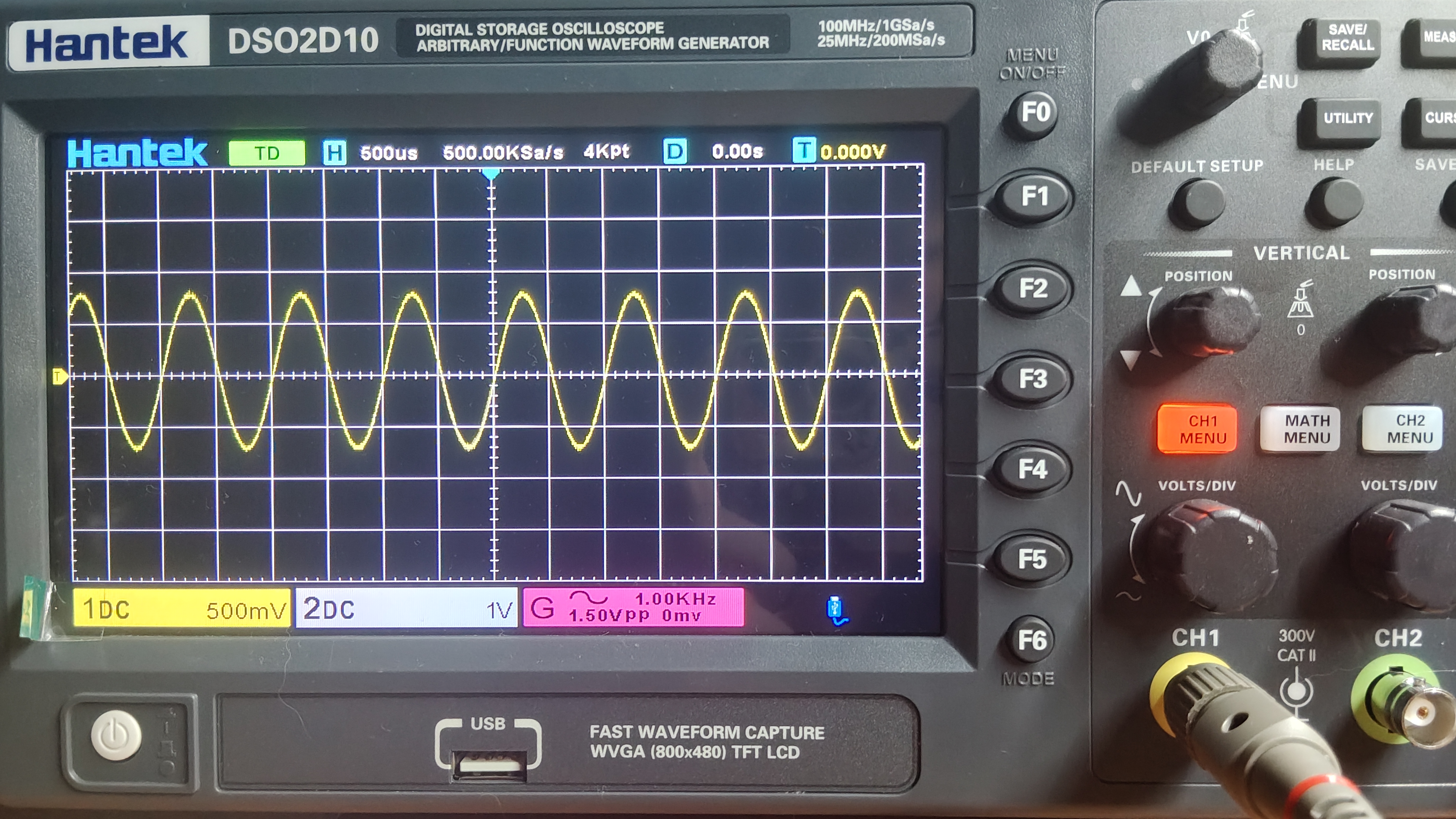
The two captures correspond to the same acquisition. The important part here is that the waveform is no longer confined to the oscilloscope display — the raw samples are available to the rest of the measurement pipeline.

This first capture is still very much an experiment rather than a finished driver. The next things to figure out are the conversion from raw samples to volts, reconstruction of the time axis, the meaning of the metadata, acquisition settings, and eventually continuous capture.

The same interface could also be used to automate measurements, collect datasets, perform custom signal processing, and build repeatable measurement procedures around the instrument.

The basic path already works:

Hantek → USBTMC → SCPI → Python → NumPy → measurement pipeline.

Not bad for a gifted oscilloscope.

Materials

The complete collection of instrument utilities is available in the tools repository.